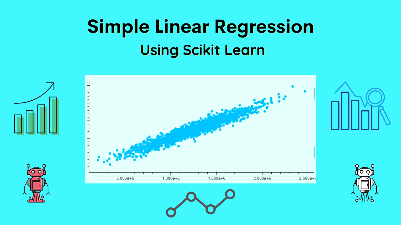
Linear Regression for Data Science

Linear Regression is a basic Machine learning Algorithm, which tries to build a relationship between two variables through a linear equation.

y\quad =\quad \alpha \quad +\quad \beta x

One variable in the linear equation called the independent variable and the other one called the dependent variable.

First should determine the strength of the relationship between the desired variable before trying to fit a linear equation to any given data.

Fitting a linear equation to the given data will not serve the purpose If there is no significant relationship between the two variables.

Scatter Plot and Correlation coefficient are the most common ways to determine the strength of the relationship between the desired variable.

Scatter Plot gives us a visual idea about the relationship between the two or more variables.

The correlation coefficient gives us a numerical measure of the relationship between the two variables.

A Linear Regression model contains the following form of the equation where X is the independent variable and Y is the dependent variable (because Y depends on X)

Y\quad =\quad a\quad +\quad bX\quad +\quad \varepsilon

Whereas b is the slope of the Straight line, X is the intercept(i.e. the value of Y when X=0) and e is the random error.

Assumption of the Linear Regression Model:

Linearity: There is a linear relationship between the dependent(X) and independent(Y) variables.
Homoscedasticity: The Variance of the Residual can be the same for any value of X (i.e Random Error which is in the form of normal independent distribution)
Independence: The successive observations of the independent variable X are independent of each other.
Normality: It can be used for any value of X, Y which is the form of Normal Distribution.

Least Square Estimation:

The Simple Linear Regression uses a single independent variable (X) and dependent variable(Y), which has a general form of equation Y = a + bX + e.

The Least Square Estimation method applied to estimate the regression coefficient a & b which are intercept and slope of the straight line respectively and based on both the estimated coefficient, it decides on the best-fitted line.

The simple principle on which it works that try to decrease the vertical deviation of each point from the best-fitted line.

The next step is to square the deviation and adds it all up so the risk of canceling the positive and negative values can be ruled out.

Adequacy of the Regression Model:

Residual Analysis:

Once a regression model gets fitted it is always helpful to plot the Residuals (the difference between the fitted line to observed values) in time sequence, against Y values, or against X Values.

It helps to get an idea of the distribution of the residuals (to know whether it is normally distributed or not)

At the start of our study of simple linear regression, we assume that the Random error is the Normal Independent distribution.

If the assumption does not hold a model then fitting a linear regression model to the said data will not be fruitful.

R Code for Simple Linear Regression

#Load the data like Train and Test datasets
#The values must be numeric and NumPy arrays for the linear regression model

# Read the csv dataset file
train <- read.csv("data.csv")

# Sample the data In Train and Test Dataset
train_data = train[sample(seq(1,200),0.8*nrow(train)),]
test_data = train[sample(seq(1,200),0.2*nrow(train)),]


# Train the model using the training sets and check the score
Linear_model <- lm(y_variable_train_data ~ ., data = train_data)


# Get The Statistical Summary of data
summary(linear_model)


#Predict Output
prediction = predict(linear_model, test_data)


# Print the predicted output
print(prediction)


# find the root mean square error of the liner model
RMSE_of_model = rmse(test$y_variable_test_data, prediction)

Python Code for Simple Linear Regression

# Import the Python Libraries for linear regression
import numpy as np
from sklearn.linear_model import LinearRegression


# Create a numpy array data
x = np.array([2, 10, 20, 30, 42, 65, 72]).reshape((-1, 1))
y = np.array([7, 14, 18, 27, 33, 42, 55])


# Build the regression model on x and y array matrix
model = LinearRegression().fit(x, y)


# After the model fitted, you can check the efficiency of the model and it's working capability.
# You can get the coefficient of determination (𝑅²),  intercept, and Slope with specific functions.


# Get the 𝑅² of model
squ_of_r = model.score(x, y)
print('coefficient of determination:', squ_of_r)


# Get the intercept of line
intercept = model.intercept_
print('intercept of model:', intercept)


# get the slop of line
Slope = model.coef_
print('slope of model:', Slope)


# To get the prediction of data based on test data
Prediction = model.predict(x)
print('prediction of responce variable:', Prediction, sep='\n')

Conclusion

In the end, Linear regression is a very efficient model which contain simple and multiple approaches for numerical data prediction.

Simple linear regression makes the linear modeling very easy to understand and apply for a very wide variety of data.

A Complete Guide on Linear Regression for Data Science

Assumption of the Linear Regression Model:

Least Square Estimation: