Simple Linear Regression Using Scikit Learn

In this post, you are going to learn the importance of linear regression and how to implement it using Scikit learn in python.

Linear Regression is a supervised learning technique used to perform predictions on numerical data.

This is a foundational machine learning technique that can serve as a first step into a more complicated algorithm such as Random Forest or Support Vector Machine.

Linear Regression Simulations

There are different types of regression, but for this introductory tutorial, we’ll try doing linear regression from scratch. Linear regression has a really nice property called the “constancy property”.

A set of data points, if added to a scatter graph with their corresponding fitted line, should pass through a single point – the origin.

I’ve written before about how I like building Monte Carlo models. I love simulations because they let you try different values of the key unknowns in your model and make more clear the assumptions made in a model.

They also make the results of your modeling effort more tangible and can help you gain an intuitive sense of what happens when different assumptions in your model are violated.

Simulations are software packages that follow a set of instructions to make something happen.

In this post, I’ll walk you through a simulation example of linear regression using bootstrapping.

There are plenty of examples that show you how to simulate data from a linear regression model using various functions in R (like nls() ).

But that didn’t really help me understand what’s going on behind the scenes. Below, I’ll work through the steps manually.

This will give you some insight into how random sampling builds on theoretical foundations and gives you the power to run analyses in situations where simulating with functions would be inconvenient.

As a quick side note: real data is much too dirty to work within this way and you should always examine results on real data.

I am using simulated data because it’s really easy to analyze, but that means all the mistakes and inaccuracies are mine, not yours! Good news though: I won’t mind at all if you misuse my code, so long as you cite me

Many people are comfortable fitting even simple linear regression models. But few people actually think about the assumptions of the model as they work with them and as a result.

I think it’s important for everyone to understand how to not just fit models, but also to create good simulations of what those models would produce.

The field of applied statistics is filled with statistical models that are used to analyze data in a variety of applications including engineering, economics, medicine, and the natural sciences.

Assumptions of Simpler Linear Regression

The assumptions of simpler linear regression are so basic that they rarely introduce any problems.

Following are the important Assumptions of Simpler Linear Regression we need to build in the model:

1. Linear relationship:
2. Independence:
3. Homoscedasticity:
4. Normality:

The equation can be simplified to y=bᵢx, where ᵢ is the variance in x. It is important to remember that s and r should be known.

The assumptions of linear regression are different from those of most other statistical methods because they are related to the structure of the model more than to the distribution of errors.

Linear regression assumes that there is a linear relationship between the response variable (y) and the predictor variable.

This linear relationship may be further described by one or several straight-line functions. Moreover, the relationships described by these functions need to be monotonic in x.

There are a few possible ways to define what it means for a relationship to be monotonic, so I will briefly describe them here.

Imagine x and y are in R and this would define a line in R². When assuming monotonicity, you should check that all points along both sides of the line (x=0 and x>0) generate values for y that increase with increasing x.

If this holds for every point in R, then you get a positive monotonic regression line.

Alternatively, you might want to require that there are points where y increases with increasing x (a monotonically increasing function), but there is either no point where y decreases with increasing x (a negatively monotonic function), two points that define the same line or that there is at least one point on each.

Working Out the Regression Equation

Start by defining a new variable w for our linear regression. This is the handle for what we’re going to call “weight.”

If you have more than one predictor variable, just choose a number to have the first one.

Next, any of your variables can be plugged into F(x), or f, to stand for a linear function.

In this equation, summation stands for adding each term together. Our example’s F(x) would be 10x, where 10 is the weight and x is the input from some other variation on linear regression.

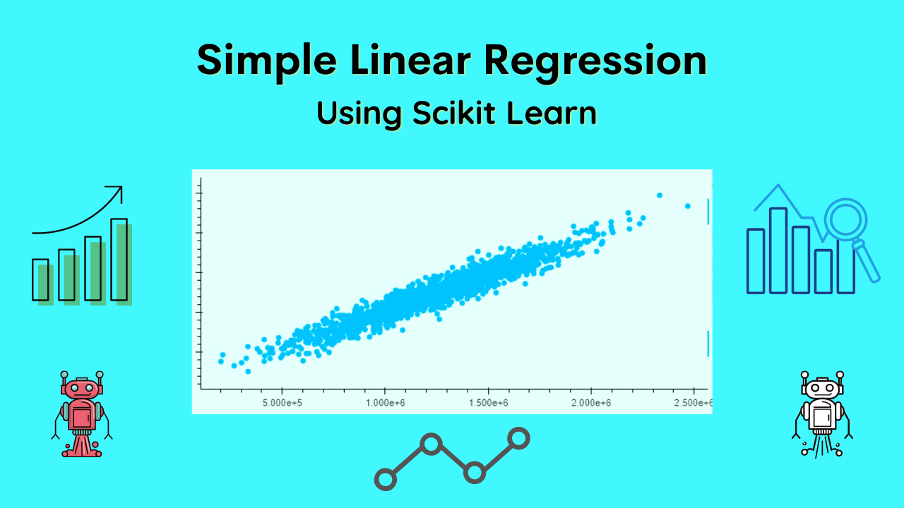
Simple Linear Regression Using Scikit Learn in Python

In the below case study of USA housing data, we are going to perform simple linear regression Using Scikit Learn Python.

For the below case study you can use the dataset from this link – Download

Step 1: Importing the required python libraries

## Import The libraries

import pandas as pd
import hvplot.pandas

Use Scikit Learn for Simple linear Regression Model
from sklearn.linear_model import LinearRegression

Step 2: loading the data from a CSV file

## Read the Data
df = pd.read_csv('USA_Housing.csv')
df.head()

Step 3: Creating the dependant and independent variable for modeling

X = df[['Avg. Area Income', 'Avg. Area House Age', 'Avg. Area Number of Rooms', 'Avg. Area Number of Bedrooms', 'Area Population']]

y = df['Price']

Step 4: Splitting the data in Train & Test

##Train Test Split 

from sklearn.model_selection import train_test_split

X_train, X_test, y_train, y_test = train_test_split(X, y, test_size=0.6, random_state=49)

Step 5: Data Scaling and normalization

from sklearn.preprocessing import StandardScaler
from sklearn.pipeline import Pipeline

pipeline = Pipeline([
    ('std_scalar', StandardScaler())
])

X_train = pipeline.fit_transform(X_train)
X_test = pipeline.transform(X_test)

Step 6: Building the Linear Regression Model

from sklearn.linear_model import LinearRegression

MachineBrain = LinearRegression(normalize=True)
MachineBrain.fit(X_train,y_train)

Step 7: Finding the Coedicient and intercept of the model

m = MachineBrain.coef_  
c = MachineBrain.intercept_

Step 8: Predicting the output based on Coedicient and intercept of the model

y_predict = m*3+c
y_predict

Step 9: Predict the Data (X_test) based on a regression model

y_predict = MachineBrain.predict(X_test)
y_predict

Step 10: Visualizing the Test data and the Predicted Data

pd.DataFrame({'True Values': y_test, 'Predicted Values': y_predict}).hvplot.scatter(x='True Values', y='Predicted Values')

Output: Simple linear regression

Conclusion

In a summary, we have concluded that linear regression is a very powerful tool for drawing insights from our data, and Scikit learn is a very powerful library for it.

Linear regression can be used to predict future events based on correlations with the past datasets and python is very crucial in terms of using regression and Scikit learn.

There are three things you need to keep in mind while testing your research – the way the independent variable affects what you are observing, the distribution of your dependent variable, and whether or not your dependent variable is random or predictable?

Recommended Articles:

Gradient descent Derivation – Mathematical Approach in R

What Is A Statistical Model? | Statistical Learning Process.

What Are The Types Of Machine Learning? – In Detail

What Is A Supervised Learning? – Detail Explained

A Complete Guide On Linear Regression For Data Science