Gradient descent Derivation – Mathematical Approach in R

In this article, we are going to see the mathematical approach of Gradient descent and its derivation using r programming.

What is Gradient Descent?

Gradient descent is the process of going downward in a slop step by step with a learning rate to reach the global minimum.

It is an optimization algorithm to find solutions or minimize that minimize the value of a given function.

Here we will try to understand the gradient descent first with an example of mountains and valleys.

Suppose you go in the mountain for trekking and after trekking, you reach the top and now you want to go to the lowest point of the valley. So for that first, you need to find the exact lowest point where that exists.

You look around to find out which is the optimal way and the path with small steps you can reach the bottom.

You then do that again and again until you reach a point where every direction is uphill. You have now found minima, but it might not be the lowest point in the mountains.

Now, you are guaranteed to reach the bottom if there was only one valley (convex function), but you might get stuck in a valley that is sub-optimal if there were multiple valleys scattered throughout the mountains (non-convex function).

Gradient descent is analogous to you looking for the downhill direction; it starts at an arbitrary point and moves in a downward direction or the negative direction of the gradient.

After several iterations, it will eventually converge to the minimum.

Learning rate

It is the count of functions that is moved every step from local minima to global minima.

Learning rate is defined mostly in decimal points to show the learning rate of the algorithm.

The learning rate is simply how large a step we take too large of a step-size will result in us bouncing around and never reach the bottom.

Local Minima

It is the best starting point to each at the global minimum with very little effort.

For Example, if you have a function f(X) and you want to find the exact point where the function is minimized itself.

Local minima are the best solutions or points in a corresponding neighborhood; in other words, these are pretty good solutions but they are not the best.

Global Minima

The global solution is the best solution overall because that you get after several iterations with low MSE and optimized output.

The concept of local minima is related to the concept of convex and non-convex functions; convex functions are guaranteed to have a global minimum or solution, while non-convex functions do not have that guarantee, which results in models obtaining local minima.

The best we can do is run an optimization algorithm (e.g. gradient descent) from different starting points and use the best local minima we find for the solution to reach a global one.

What is Stochastic gradient descent (SGD)?

It is a variant of gradient descent and simply performs the gradient step on one or a few data points as opposed to all the data points), which allows us to jump around and avoid getting stuck in local minima.

It is computationally more efficient and may lead to faster convergence, but results in noisier results.

Mini-batch stochastic gradient descent (mini-batch SGD) randomly chooses batches of data points (between 1 and 1000 or 10 to 10,000) and then performs a gradient step.

This process helps to reduce noise and speed up training Gradient descent is an optimization algorithm used to minimize some function (cost function) by iteratively moving in the direction of down as negative of the gradient.

By moving in the direction of the negative gradient, we slowly make our way down to a lower point until we get to the bottom (local minima).

We use gradient descent to update the parameters of our model and to find the parameters that minimize the cost function.

Cost function

It is an advanced form of the loss function that we can define based on loss function which comes from the data points or the error-ness in a tanning data set.

So before understanding the cost function getting the normal view of the loss function is very significant to solve any machine learning problem.

The loss function is probably a function used to describe the forms of data, level of prediction, and regularization in the model.

Similarly, the Cost function comes from the loss function which is the mean of the loss function or the error function in the model.

Gradient Descent Derivation In R

The below code will help to understand the gradient descent derivation implementation to solve any type of machine learning problem if that needs optimization.

We will implement gradient descent with the following simple steps:

1. load the libraries

Install and load the required libraries in r studio for implementation.

library(dplyr)
library(ggplot2)
library(plotly)

2. Loading the data

Load the data to perform gradient descent on it. you can download this dataset here

ads = read.csv("Advertising.csv")

3. Sampling of data

Sample the data in two different datasets including training and test form

ads_training = ads[sample(seq(1,200),0.8*nrow(ads)),]

ads_training = ads[sample(seq(1,200),0.2*nrow(ads)),]

4. Define Variables

Define a few variables before creating a function of gradient decent

m1 = 0.5
c1 = 10

Plotting the variables to see the data point in a training data

{{plot(ads_training$TV, ads_training$sales, xlab = "TV",ylab = "Sales") abline(c1,m1)}}

5. Error Fucntion

Create a mean Square Error Function to define error in gradient descent

mse = function(x , y , m ,c){
  yhat = m * x + c
  error = sum((y - yhat) ^ 2) / length(x)
  return(error)
  
}

sample_x = c(1:5)
sample_y = c(10,20,30,40,50)
m = 5
c = 1

mse(sample_x,sample_y, m, c)

iterations = 100
cspace = seq(1,10, length.out = iterations)

mspace = seq(-0.6,0.6, length.out = iterations)

zspace = c()

for(i in mspace){
  for (j in cspace) {
    zspace = c(zspace, mse(ads_training$TV, 
                           ads_training$sales, 
                           i, j))
  }
}


zmat = matrix(zspace,iterations,iterations)

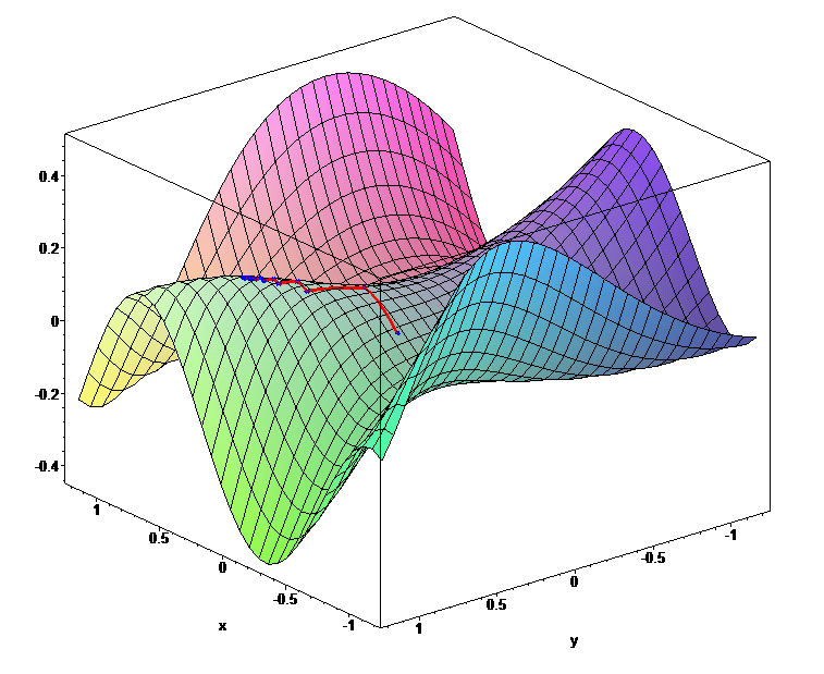
plot_ly(x = mspace, y = cspace, z = zmat) %>% add_surface()

The output of the above code:

6. Model Building

A simple example of building a linear model

x = rnorm(100)
y = 0.05 * x
df = data.frame(x=x,y=y)

lm(y~x,data=df)

7. Gradian decent Derivation

Implementation of Gradian decent to reach global Minima

m = 100
#m = 10
alpha = 0.01
#alpha = 0.2      # learning 
iterations = 100  # we can increase the iteration to get the global minimum

for(i in seq(1,iterations)){
  df = mutate(df,xy_vals = x*y)
  df = mutate(df,mx_square = m * (x^2))
  df = mutate(df,xy_minus_mx2 = xy_vals - mx_square)
  m_gradient = -2/nrow(df) * sum(df$xy_minus_mx2)
  
  m = m - alpha * m_gradient 
}
print(m)

8. Calculating the error value for every M value

m = 100
#m = 10
alpha = 0.01
#alpha = 0.2           # learning rate
iterations = 1000      # we can increase the iteration to get the global minimum

errors_vals = c()

for(i in seq(1,iterations)){
  df = mutate(df,mx_vals = m*x)
  df = mutate(df,y_mx_vals = (y - mx_vals)^2)
  curr_error = sum(df$y_mx_vals) / nrow(df)
  errors_vals = c(errors_vals,curr_error)
  df = mutate(df,xy_vals = x*y)
  df = mutate(df,mx_square = m * (x^2))
  df = mutate(df,xy_minus_mx2 = xy_vals - mx_square)
  m_gradient = -2/nrow(df) * sum(df$xy_minus_mx2)
  
  m = m - alpha * m_gradient 
}
plot(errors_vals)

9. Implementation of Equations

Implementing the derivative equation of gradient descent in r code

y = 0.05 * x + 100
df = data.frame(x=x,y=y)
alpha = 1 / nrow(df)
m = 0
c1 = 0
iterations = 500

m_vals = c(m)
c1_vals = c()
errors_vals = c()

for (i in seq(1,iterations)){
  m_vals = c(m_vals,m)
  c1_vals = c(c1_vals,c1)
  df = mutate(df, e = (y - m * x - c1)^2)
  df = mutate(df,msigma = (x * y)-(m * x^2) - (c1*x))
  df = mutate(df,csigma = y - m * x - c1)
  errors_vals = c(errors_vals,sum(df$e)/nrow(df))
  m_gradient = -2/nrow(df) * sum(df$msigma)
  c1_gradient = -2/nrow(df) * sum(df$c1sigma)
  m = m - alpha * m_gradient
  c1 = c1 - alpha * c1_gradient
}

print(list(m=m, c=c1))

Conclusion

In the above article, we have explored the derivation of gradient descent using r programming.

There are few languages like python, java, and others you can use to implement the gradient descent and as well its derivation.