Principal Component Analysis by Sklearn – Linear Dimensionality Reduction

In this article, you will learn how to do principal component analysis using the Sklearn python library on high-dimensional data.

The results of the PCA will be visualized using the seaborn and matplotlib libraries.

The Sklearn Principal Component Analysis module makes it easy to use PCA for dimensionality reduction and data visualization.

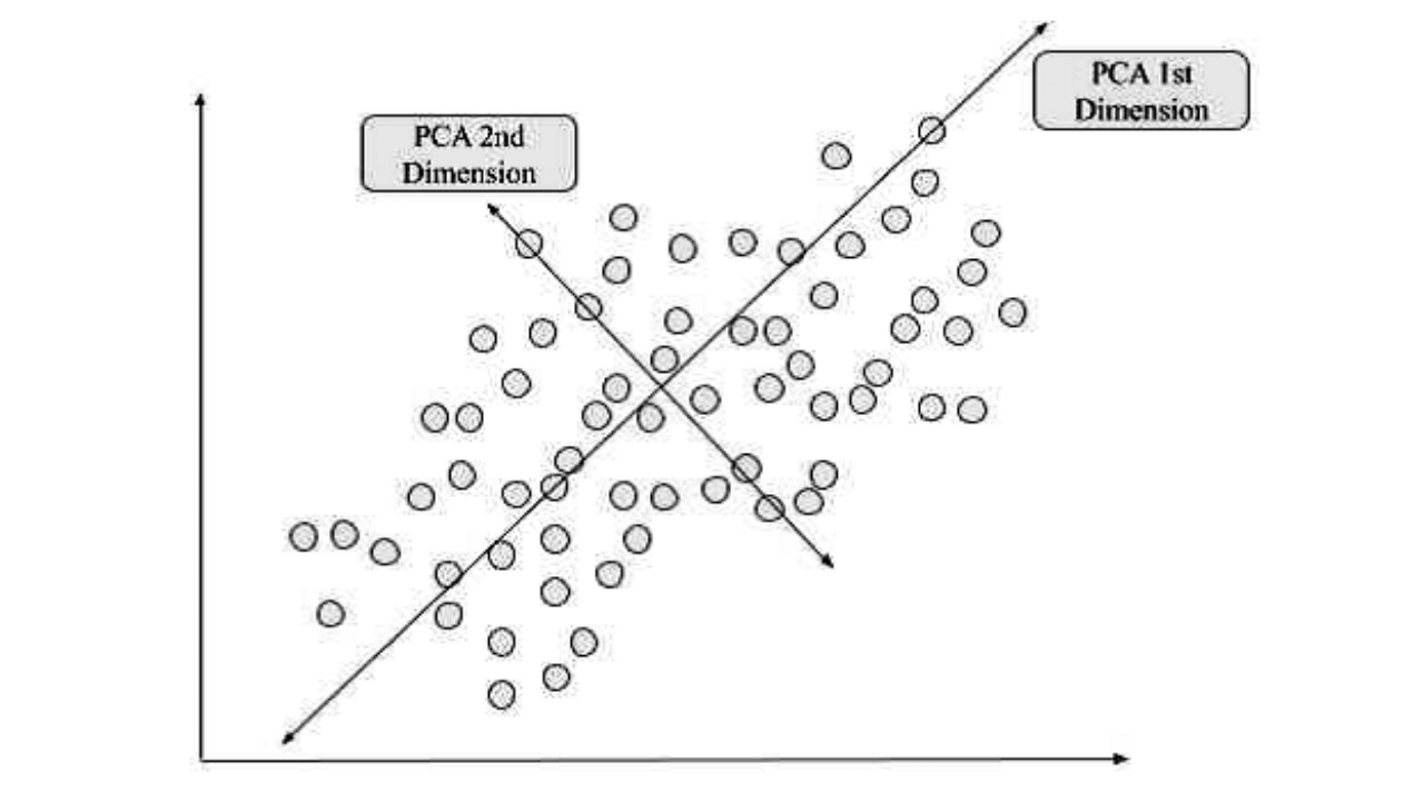
Principal component analysis (PCA) is a statistical method used to reduce the dimensionality of data by transforming it into a new set of variables called principal components, which are linear combinations of the original variables that maximize the variance in the data.

The new set of variables can be used to represent the original data in lower-dimensional space, thereby revealing patterns that would otherwise be hidden in the original data and allowing new insights to be drawn from the dataset.

PCA is one of the fundamental tools used in many machine learning applications including dimensionality reduction, feature extraction, feature selection, and model training.

Principal Component Analysis (PCA)

One of my favorite machine learning algorithms is Principal Component Analysis.

Often used with data visualization and exploratory data analysis, PCA seeks to project a dataset onto a lower-dimensional subspace that preserves as much information as possible.

In order to achieve such an ambitious goal, we must first transform our data in ways that allow us to take advantage of different useful properties, such as linearity and variance homogeneity.

Note: This post assumes knowledge of linear algebra, eigenvalues/eigenvectors, statistical concepts such as mean and variance (and their calculation), and familiarity with multidimensional arrays;

If these terms are new to you then it might be helpful to have a look at some introduction material before continuing.

Why PCA?

In addition to its excellent scalability, one of Scikit-learn’s strengths is in modeling complex datasets using linear methods.

In machine learning, these linear models are known as unsupervised learning algorithms, because they can find patterns in data without relying on a teacher or human expert.

The two main types of unsupervised learning methods that we will look at here are clustering and principal component analysis (PCA).

Clustering works by grouping similar elements together while PCA finds features that can summarize a dataset by capturing most of its variance.

We will focus on PCA since it allows us to deal with many numerical attributes.

Related Article: What is Unsupervised Learning in Machine Learning?

PCA Using Singular Value Decomposition

PCA SVD in python Find eigenvalues and eigenvectors of a matrix, perform Singular Value Decomposition (SVD) and convert an array to its diagonal.

If a lower-dimensional subspace exists within a set of variables, then singular value decomposition finds matrices U and V such that X=USV* or Y=UV* where * indicates complex conjugate transpose.

These operations are related to whitening or decorrelating data. This is commonly used for dimensionality reduction and sometimes feature extraction when doing statistical analysis on large amounts of data using covariance/correlation analysis

It also works well when you want to find similar items based on co-occurrence frequencies.

What is Input Data in PCA?

PCA is a dimensionality reduction technique that projects data into a lower-dimensional space.

This is done by analyzing input data’s correlations to project it to a lower-dimensional space.

PCA also centers and scales data for each feature before applying Singular Value Decomposition (SVD).

The principal component analysis differs from similar techniques, such as independent component analysis or canonical correlation analysis, because it emphasizes revealing structure in input data without trying to explain it.

In other words, the principal component analysis aims to find directions of maximal variance which are not necessarily correlated with any obvious pattern of variables.

Finding these structures can help you better understand your data in terms of underlying factors you were previously unaware of.

For example, imagine that your dataset contains values between 0 and 1 on two continuous features.

We have 100 data points and we want to create a model for predicting whether an observation belongs to class 1 (0) or class 2(1).

Our model would need at least 3 parameters: mean value of both features in case we want observations to be close to zero when they belong to class 1, mean value in case they belong to class 2 but slightly different than zero since there are two classes; all three parameters could be used together.

How does PCA work?

It is a linear dimensionality reduction technique used to remove the high dimension from the data.

In layman’s terms, it transforms your high-dimensional data into a low-dimensional space.

What does that mean? It means you can use PCA to take something complicated and make it easy for people to understand.

It does that by creating new variables (called principal components) from your original data that are simpler in nature than your original variables.

As a result, when you display your original data on top of these new principal components, they tell most of your story while being easier to comprehend.

Having said all that, what exactly do we mean by linear dimensionality reduction? Well… dimensions can be thought of as directions in which we could move our point around.

We can represent two dimensions with an x/y plane where an increase in value along one axis is associated with a decrease in value along another axis.

PCA turns your high-dimensional data into a new set of coordinates (your principal components) that are still tied to your original data and allows you to visualize most of its variance while being easier to comprehend.

What is Output Data in PCA?

Principal component analysis, like all linear dimensionality reduction techniques, reduces a data matrix to a lower-dimensional space.

The data is centered but not scaled before projecting it to a lower-dimensional space.

The number of components (or principal components) that are retained in a given projection depends on how much of the total variance in your data is explained by those components.

If you are using PCA for predictive modeling then you want to retain as many components as possible so that you can best predict future samples in your training set.

There’s no hard and fast rule about what constitutes enough since there will always be some remaining variance in your data.

You just have to choose an appropriate value based on what you’re trying to accomplish with PCA.

For example, if you only have 10 features and 2% of the sample variance is captured by 10 principal components then you should stop there even though there may be more information present.

How can I apply PCA to my data?

The principal component analysis is a technique for reducing dimensions. It’s useful when your data is high-dimensional.

In particular, it can often help remove noise in your dataset while retaining most of its structure.

But PCA isn’t a silver bullet, and using it carelessly can lead to disastrous results! Make sure you understand exactly what PCA does before trying to use it on your own data.

In many cases, there are better techniques for dimensionality reduction than PCA (for example, if there are nonlinear relationships between features).

However, when used correctly—and combined with other tools—PCA provides an extremely valuable function.

How do I apply sklearn’s implementation of PCA?:

If you want to run sklearn implementation of principal component analysis on your data, simply follow these steps:

Step 1: Import scikit-learn’s (sklearn) implementation into python2 or python3, This uses NumPy.

import numpy as np 
from sklearn import decomposition 

Step 2: Alternatively, you could create a new file for your code and paste it into that file like so:

from sklearn import decomposition 

Step 3: Read in your data.

Remember that in order to use PCA, your input data needs to be centered about zero! You can ensure your data is centered by taking each feature vector and subtracting each row’s mean across all examples within each feature vector.

X = [[1, 2], [5, 2], [7, 5]] 

print(X) 

Y = np.array([[0], [1], [2]]) 

Step 4: Calculate SVD.

svd = decomposition.PCA(n_components=2).fit(X) 

vsrpca = svd.transform(X) 

Step 5: Use scatter_matrix function to plot results

scatter_matrix(vsrpca, label='target') 

plt.xlabel('First principal component') 

plt.ylabel('Second principal component') 

Don’t forget to save your original variables and their transformed counterparts! Save them both somewhere safe; after applying principal component analysis, they’ll be more meaningful to you because they’re easier to interpret.

Step 5 will result in more information being displayed on your screen; namely two graphs showing how certain attributes correlate with one another.

The first graph plots how your input variables relate to one another along one axis.

The second graph shows how they relate along another axis.

Limitations of PCA

PCA is a powerful technique, But it is not the only one, Carefully evaluate whether or not PCA is appropriate for your data and determine if it actually makes sense before proceeding to use it.

In many cases, other methods of dimensionality reduction such as ICA or t-SNE provide greater insight into what’s going on with your data than PCA does (for example, in natural language processing).

However, when used correctly, combining PCA with other tools can be extremely valuable!

How to Perform Principal Component Analysis using Sklearn?

PCA is a popular technique used for data compression and exploratory analysis.

The input data can be seen as a matrix $X = \begin$ with each column being a set of correlated features and each row being an example/object.

The goal of PCA is to project these samples onto a new lower-dimensional space such that:

1) Each sample still has maximum variance in its original feature space,

2) The samples are spread out (as much as possible) in their new feature space.

For Python we recommend using scikit-learn, which provides implementations of many Machine Learning algorithms.

As you may have guessed from sklearn’s name, it uses SciPy’s linear algebra functions under the hood.

But fear not: you don’t need to know anything about linear algebra to use the Sklearn machine learning library for principal component analysis.

First, import NumPy (required by almost all other libraries) and SciPy (which actually contains most of scikit-learn):

import NumPy
import SciPy

Next, import matplotlib so that we can visualize our results:

import matplotlib

Finally, let’s load up a dataset I found on Kaggle after doing a Google search for iris datasets.

Let’s say we want to predict whether or not someone smokes given information like age and gender.

One good strategy might be to find if there are correlations between smoking and any numerical features in your data (like age).

This can easily be done using PCA, We won’t cover how to interpret these values since it would take us off track too much.

Conclusion

PCA is a linear dimensionality reduction technique. It is a generalization of discrete Fourier transform (DFT).

It finds eigenvectors and corresponding eigenvalues of the data covariance matrix, centered data doesn’t need to be scaled before applying SVD.

Although PCA is not suitable for a large number of features (n<10000), it is good for analyzing datasets with small sample size.